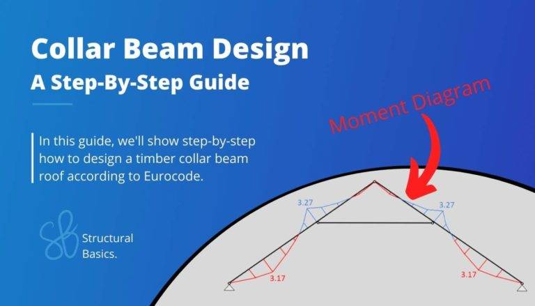
Steel to Timber connection – Beam to beam – An example of a flat roof connection
One key aspect of dimensioning timber elements such as beams and columns is the timber connection design.
The structural elements can be well verified for bending, shear, deflection, buckling, etc. but when designing the connection it can happen that the width or height of the cross-section is too small to fit all fasteners and the Cross-section needs to be increased.
So it does make sense to keep the utilization of the elements a bit lower in the initial design phase.
Before we get into the nerdy calculations, let’s ask: What is a steel to timber connection?
A steel to timber connection is a connection built up by multiple layers of steel plates and timber elements like beams, panels, etc. The forces are transferred to each layer by fasteners like nails, bolts, screws which are mostly subjected to lateral forces.
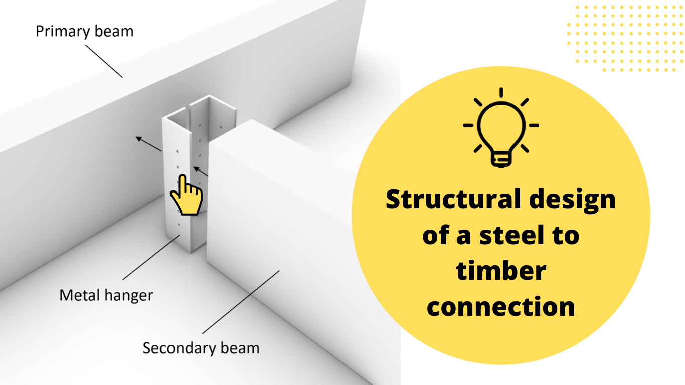
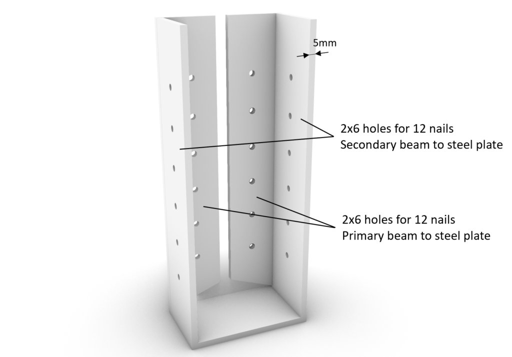
The following picture is showing the connection we are designing in this tutorial.
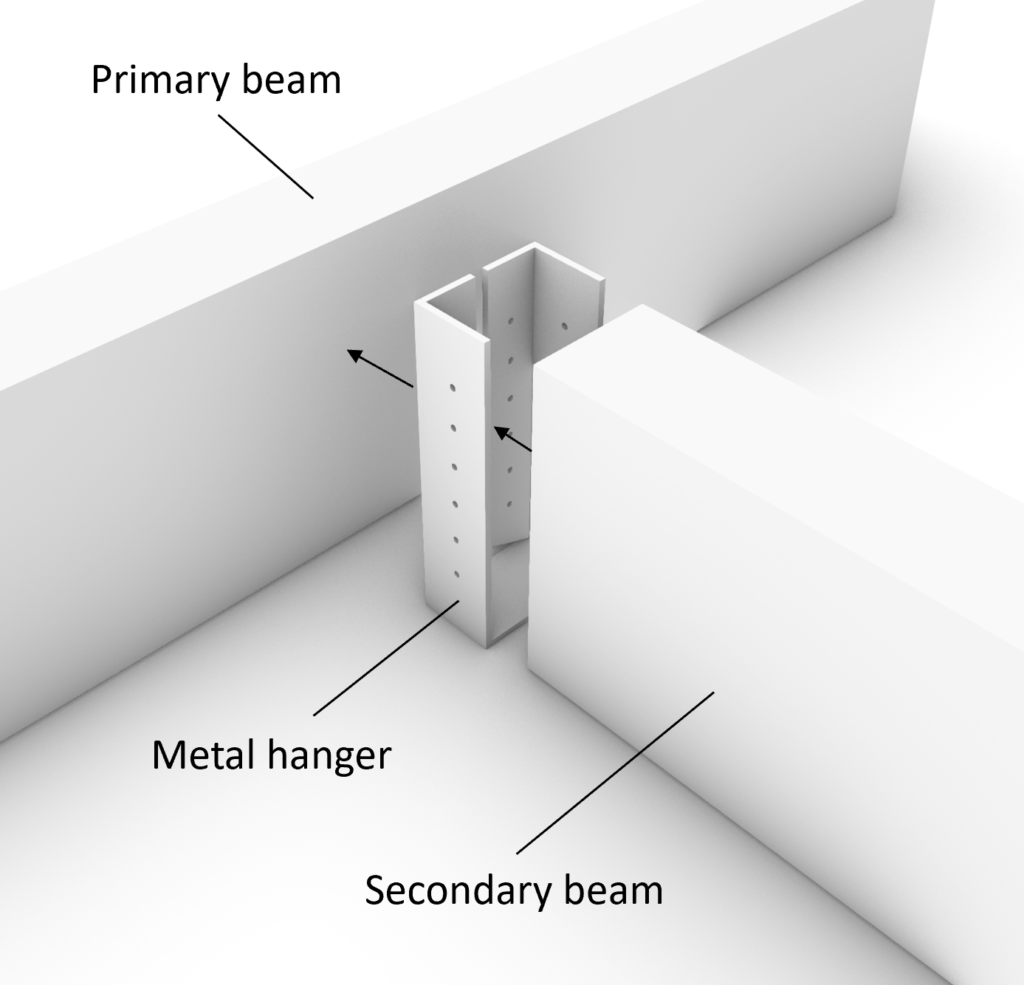
This connection can be used for a flat roof connecting primary to secondary beams.
So let’s have quick look at what we are doing in this post:
- Static system of the beams and connection type
- Loads acting on the connection and how to derive them
- Load combinations
- Timber beam material
- Modification factor $k_{mod}$
- Partial factor $\gamma_{m}$
- Beam cross-section width and height
- Design of connection – secondary beam to steel plate connection
- Design of connection – steel plate to primary beam connection
- Model or drawing of connection
Static system of the beams and connection type
It is very important to understand the static system of the beams and how they are connected to each other in order to choose the correct connection and connection calculation.
It always helps to explain it with an example.
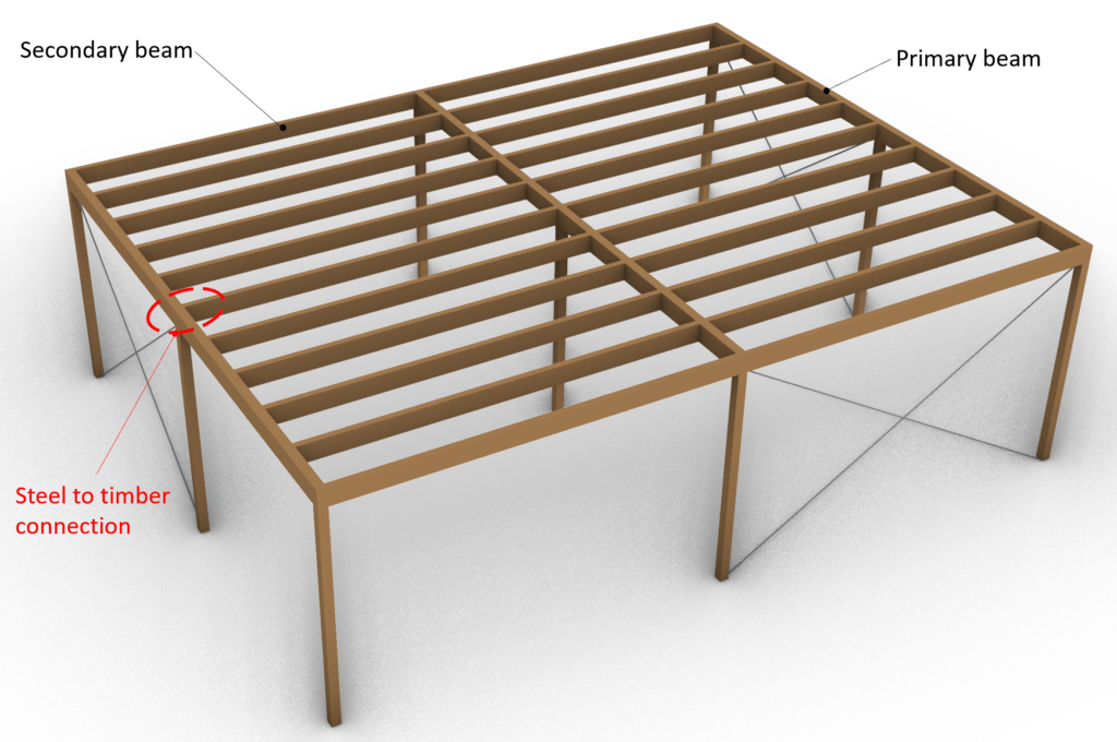
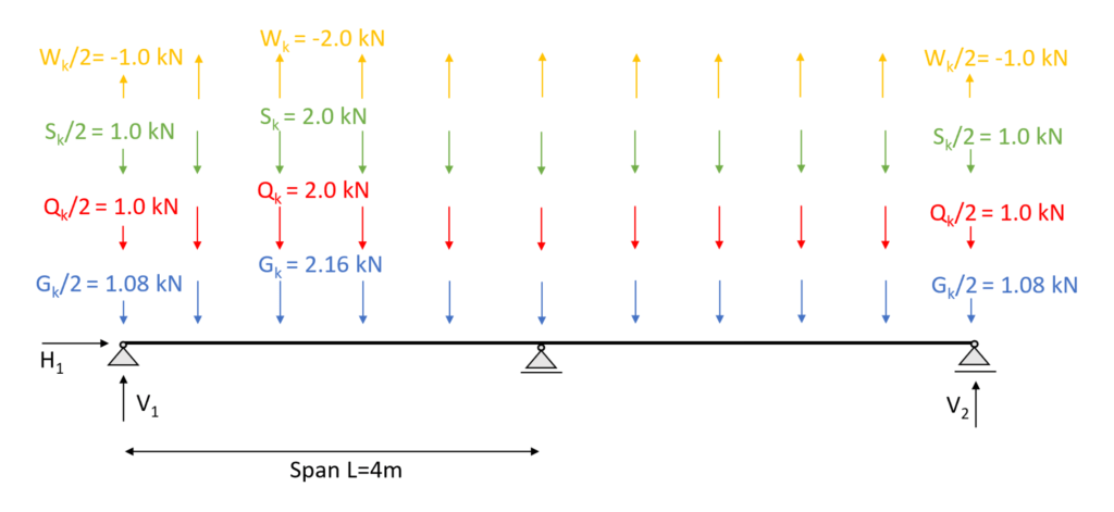
In our example, the secondary beams are simply supported and connected to the primary beams with hinged connections, while the primary beams are continuous beams supported by 3 columns.
Don’t get confused by the alignment of the supports here. We simply drew 2D supports in a 3D model and look at each element separately.
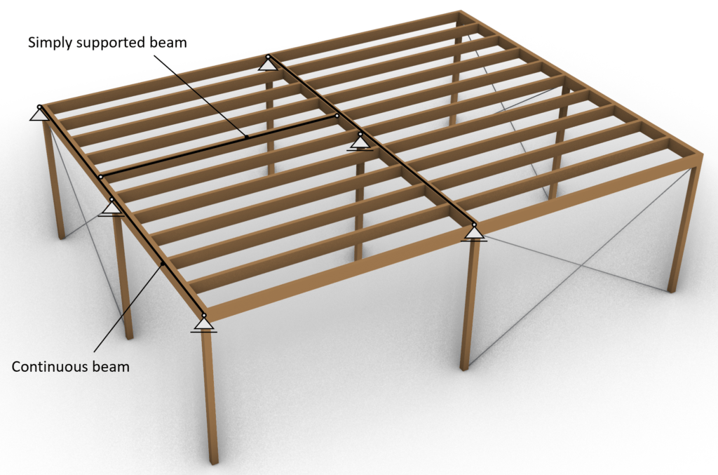
We can learn from the statics system of the beams that the connection we design is a hinge which has the following characteristics:
- allows for rotations
- Shear connection. Bending moment = 0
Loads
From the previous section we have learned that the bending moment is 0 in the connection and that the connection therefore only takes shear forces.
Those shear forces equal the vertical support forces of the simply supported secondary beam.
Luckily, we have already written an extensive article about the design of that timber beam and can therefore use the same loads. Check out the article to read more about how we assumed the loads.
| $G_{k}$ | 2.16 kN | Characteristic value of dead load |
| $Q_{k}$ | 2.0 kN | Characteristic value of live load |
| $S_{k}$ | 2.0 kN | Characteristic value of snow load |
| $W_{k}$ | -2.0 kN | Characteristic value of wind load |
The following picture presents the simply supported beam with it’s line loads applied. It can be seen that the characteristic line loads lead to the support forces shown in the table above.
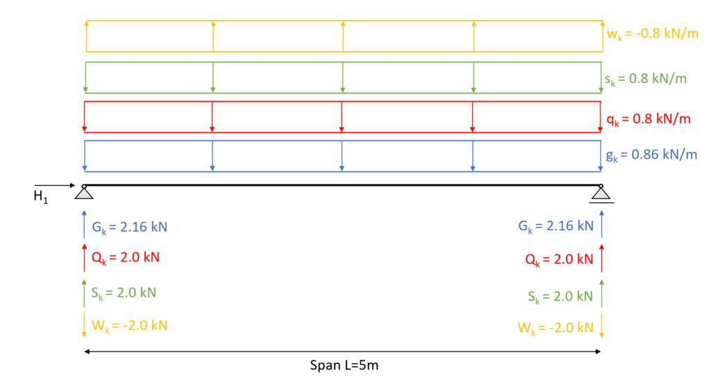
Now those support forces are used to dimension the connection but also for the further design of the primary beam. The support forces turn into point loads and can be applied to the continuous beam in order to
Okay, well, let’s get back to the topic😎.
Load combinations
In this blog post we are “only” defining the load combinations with values but if you want to read up on it more than check out our more detailed article.
ULS Load combinations
| LC1 | $1.35 * 2.16 kN $ | $2.92 kN$ |
| LC2 | $1.35 * 2.16 kN + 1.5 * 2.0 kN $ | $5.92 kN $ |
| LC3 | $1.35 * 2.16 kN + 1.5 * 2.0 kN + 0.7 * 1.5 * 2.0 kN$ | $8.02 kN$ |
| LC4 | $1.35 * 2.16 kN + 0 * 1.5 * 2.0 kN + 1.5 * 2.0 kN$ | $5.92 kN $ |
| LC5 | $1.35 * 2.16 kN + 1.5 * 2.0 kN + 0.7 * 1.5 * 2.0 kN + 0.6 * 1.5 * (-2.0 kN) $ | $6.22 kN$ |
| LC6 | $1.35 * 2.16 kN + 0 * 1.5 * 2.0 kN + 1.5 * 2.0 kN + 0.6 * 1.5 * (-2.0 kN) $ | $4.12 kN $ |
| LC7 | $1.35 * 2.16 kN + 0 * 1.5 * 2.0 kN + 0.7 * 1.5 * 2.0 kN + 1.5 * (-2.0 kN) $ | $ 2.02 kN $ |
| LC8 | $1.35 * 2.16 kN + 1.5 * 2.0 kN $ | $ 5.92 kN $ |
| LC9 | $1.35 * 2.16 kN + 1.5 * (-2.0 kN) $ | $ -0.08 kN $ |
| LC10 | $1.35 * 2.16 kN + 1.5 * 2.0 kN + 0.6 * 1.5 * (-2.0 kN) $ | $ 4.12 kN $ |
| LC11 | $1.35 * 2.16 kN + 1.5 * (-2.0 kN) + 0.7 * 1.5 * 2.0 kN $ | $ 2.02 kN$ |
| LC12 | $1.35 * 2.16 kN + 1.5 * 2.0 kN + 0.6 * 1.5 * (-2.0 kN)$ | $ 4.12 kN$ |
Timber beam material
As already explained, a structural wood C24 beam was picked for the design of the roof beam. For more details on the choices of beams, you can read up here.
The properties can either be found online from a manufacturer table or in Eurocode. We found a C24 beam from a manufacturer online with the following properties.
| Bending strength $f_{m.k}$ | 24 $\frac{N}{mm^2}$ |
| Tension strength parallel to grain $f_{t.0.k}$ | 14 $\frac{N}{mm^2}$ |
| Tension strength perpendicular to grain $f_{t.90.k}$ | 0.4 $\frac{N}{mm^2}$ |
| Compression strength parallel to grain $f_{c.0.k}$ | 21 $\frac{N}{mm^2}$ |
| Compression strength perpendicular to grain $f_{c.90.k}$ | 2.5 $\frac{N}{mm^2}$ |
| Shear strength $f_{v.k}$ | 4.0 $\frac{N}{mm^2}$ |
| E-modulus $E_{0.mean}$ | 11.0 $\frac{kN}{mm^2}$ |
| Characteristic density $\rho_{k}$ | 310 $\frac{kg}{m^3}$ |
Modification factor $k_{mod}$
If you do not know what the modification factor $k_{mod}$ is, we wrote an explanation to it in a previous article, which you can check out.
Since we want to keep everything as short as possible, we are not going to repeat it in this article – we are only defining the values of $k_{mod}$.
For the timber flat roof which is classified as Service class 1 according to EN 1995-1-1 2.3.1.3 we extract the following load durations for the different loads.
| Self-weight/dead load | Permanent |
| Live load, Snow load | Medium-term |
| Wind load | Instantaneous |
From EN 1995-1-1 Table 3.1 we get the $k_{mod}$ values for the load durations and a Structural wood C24 (Solid timber).
| $k_{mod}$ | |||
|---|---|---|---|
| Self-weight/dead load | Permanent action | Service class 1 | 0.6 |
| Live load, Snow load | Medium term action | Service class 1 | 0.8 |
| Wind load | Instantaneous action | Service class 1 | 1.1 |
Partial factor $\gamma_{M}$
According to EN 1995-1-1 Table 2.3 the partial factor $\gamma_{M}$ is defined as
$\gamma_{M} = 1.3$
Beam Cross-section width and height
As already mentioned above we are using the same cross-sectional parameters for the secondary beam that we also used in the timber beam design post.
Width w = 100 mm
Height h = 240 mm
Design of connection – secondary beam to steel plate connection
At first, we look at the secondary beam to steel plate connection and then steel plate to primary beam. Both parts need to be verified.
We use the formulas for timber to steel connections from EN 1995-1-1:2004 8.2.3 for fasteners in one shear.
For one shear plane, we look at formulas a – e from EN 1995-1-1:2004 8.2.3. In order to calculate the load bearing capacities of the connections, we need to define a few variables first.
| Diameter nails d | 5mm | Smooth nails |
| Thickness steel plate $t_{steel}$ | 5mm | |
| Nail head diameter $d_{h}$ | 8mm | |
| Length nails $l_{nail}$ | 70mm | |
| Penetration length nails $t_{pen}$ | 65mm | |
| Minimum tensile strength nails $f_{u}$ | 600 $\frac{N}{mm^2}$ | EN 1995-1-1 8.3.1.1 |
With those parameters we can calculate the characteristic embedment and withdrawal strength and the characteristic yield moment which are required for the failure modes a, b, c, d and e to calculate the characteristic load-carrying capacity.
Characteristic withdrawal strength
The characteristic withdrawal strength of the smooth nails is calculated according to EN 1995-1-1:2004 8.3.2 (8.24).
EN 1995-1-1:2004 8.3.2 (6) gives formulation for the characteristic values of the withdrawal and pull-through strengths if the penetration length is at least 12d= 60mm ($t_{pen}$ = 65mm).
| Withdrawal strength $f_{ax.k}$ | $20 \cdot 10^{-6} \cdot \rho_{k}^2 = 1.922$ | EN 1995-1-1 (8.25) |
| Pull-through strength $f_{head.k}$ | $70 \cdot 10^{-6} \cdot \rho_{k}^2 = 6.727$ | EN 1995-1-1 (8.26) |
The characteristic withdrawal strength $F_{ax.Rk}$ (EN 1995-1-1 (8.24)) is then calculated as
$min(f_{ax.k} \cdot d \cdot t_{pen}, f_{head.k} \cdot d \cdot t_{steel} + f_{head.k} \cdot d_{h}^2) = 478.58 N $
Characteristic embedment strength
With smooth nails of diameter <8mm formulation EN 1995-1-1 (8.15) is used to calculate the characteristic embedment strength.
$f_{h.k} = 0.082 \rho_{k} \cdot d^{-0.3} = 15.69 \frac{N}{mm^{2}}$
Many manufacturers actually provide this value in their datasheets and therefore do not have to be calculated.
Characteristic yield moment
For smooth nails the formulation EN 1995-1-1 (8.14) is used to calculate the characteristic yield moment.
$M_{y.Rk} = 0.3 \cdot f_{u} \cdot d^{2.6} = 1.182 \cdot 10^{4} Nmm$
As for the characteristic embedment strength, a lot of manufacturers provide this value in their datasheet. Less work for us – yaay😁.
Characteristic load-carrying capacity for nails per shear plane per fastener
From figure EN 1995-1-1 Figure 8.3 it can be seen that failure modes a, b, c, d and e apply to our connection – 1 shear plane. All parameters are defined – so let’s calculate those 5 failure modes🔥
Failure mode a
$F_{v.Rk.a} = 0.4 \cdot f_{h.k} \cdot t_{1} \cdot d = 2.04 kN$
Failure mode b
$F_{v.Rk.b} = 1.15 \cdot \sqrt{2 \cdot M_{y.Rk} \cdot f_{h.k} \cdot d} + \frac{F_{ax.Rk}}{4} = 1.685 kN$
Failure mode c
$F_{v.Rk.c} = f_{h.k} \cdot t_{1} \cdot d \cdot (\sqrt{2 + 4 \frac{ M_{y.Rk}}{f_{h.k} \cdot d \cdot t_{1}^{2}} -1})+ \frac{F_{ax.Rk}}{4} = 2.48 kN$
Failure mode d
$F_{v.Rk.d} = 2.3 \cdot \sqrt{M_{y.Rk} \cdot f_{h.k} \cdot d} + \frac{F_{ax.Rk}}{4} = 2.334 kN$
Failure mode e
$F_{v.Rk.e} = f_{h.k} \cdot t_{1} \cdot d = 5.1 kN$
The characteristic load-carrying capacity for nails is set to be the smallest resistance of the 5 failure modes.
$F_{v.Rk} = min(F_{v.Rk.a}, F_{v.Rk.b}, F_{v.Rk.c}, F_{v.Rk.d}, F_{v.Rk.e}) = 1.685 kN$
Now this is the characteristic value for 1 nail. Let’s remember us what the connection needs to resist. The design lateral load is
$F_{v.d} = 8.02 kN$
We can quickly see that we need a few nails to resist that load. Let’s increase the amount of nails to
$n = 12$
$F_{v.Rk} = n \cdot F_{v.Rk} = 20.225 kN$
.. and now we also have to transform the characteristic load-carrying capacity into the design resistance which we do like for any other timber element
$F_{v.Rd} = k_{mod.m} \cdot \frac{F_{v.Rk}}{\gamma_{M}} = 12.45 kN$
leading to a Utilization of
$\eta = \frac{F_{v.d}}{F_{v.Rd}} = 0.64$
Normally, you now also need to make sure that you fulfil all spacing requirement according to Eurocode.
We are saving that up for now since we have already written so much in this post.
But let us know in the comments below if you wish to have an explainer on how to space fasteners, nails, bolts, etc. in steel to timber or timber to timber connections.
Design of connection – steel plate to primary beam connection
We are lucky that exactly the same calculation with the same values as for the secondary beam to steel plate connection is used for the connection to the primary beam.
Or maybe we are a bit lazy and save the space🤔👀. But we can say …
With those results we design the connection which can look like …
Now we have designed our first steel to timber connection. Isn’t that cool?
I hope this blog post was useful. Let me know what you think in the comments below👍.
And see you in the next tutorial.
![Compression Verification Of Reinforced Concrete [Eurocode]](https://www.structuralbasics.com/wp-content/uploads/2024/10/Compression-verification-of-reinforced-concrete-768x439.jpg)