What Are Load Combinations And How To Calculate Them?

As buildings and structures must withstand the heaviest storms, accidental events and combined loading scenarios, engineers multiply loads with safety factors and combine different loads in so-called load combinations to make sure that the structure doesn’t collapse.

We’ll show step-by-step, how load combinations work, what different types we use and how to calculate them.

Let’s get started. 🚀🚀

What Are Load Combinations?

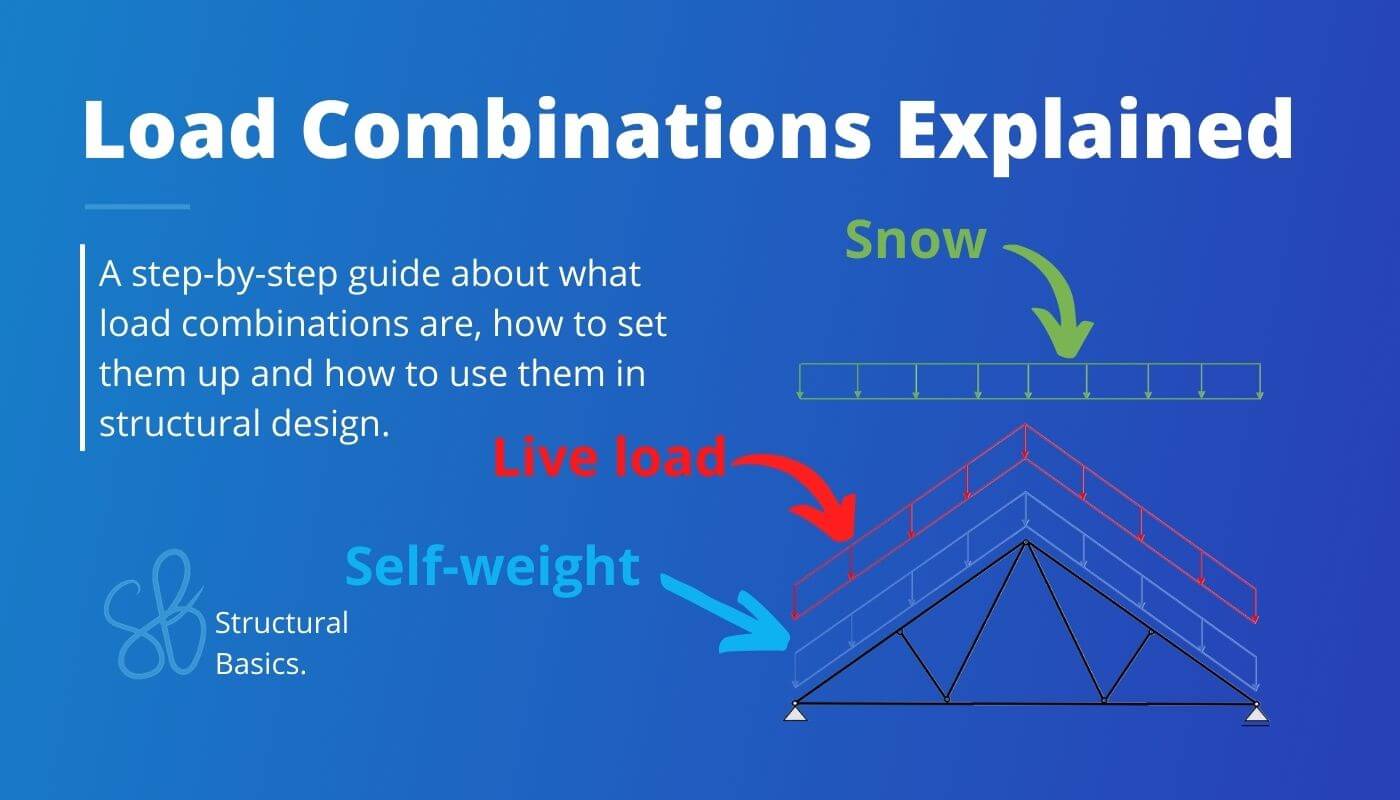
Load combinations combine different loads like snow, wind, dead, seismic and live load to represent a “real scenario”. A real scenario is for example the resulting force for a heavy wind storm. By setting up all possible load combinations we will find the worst-case scenario for a structural member which is in many cases the biggest load.

Load combinations according to Eurocode consist mostly of 3 components:

• The characteristic load value (snow, wind, dead, seismic, live load)
• Partial factor $\gamma$
• Factor for combination value of variable loads $\Psi_{0}$

Depending on the structural member, we verify usually verify for the following types of load combinations:

View this post on Instagram

A post shared by Structural Basics | Structural Engineering (@structural.basics)

We’ll show all of these 6 types of load combinations more in detail later in the article.

To understand load combinations better, we’ll explain everything with an example structure. 👇👇

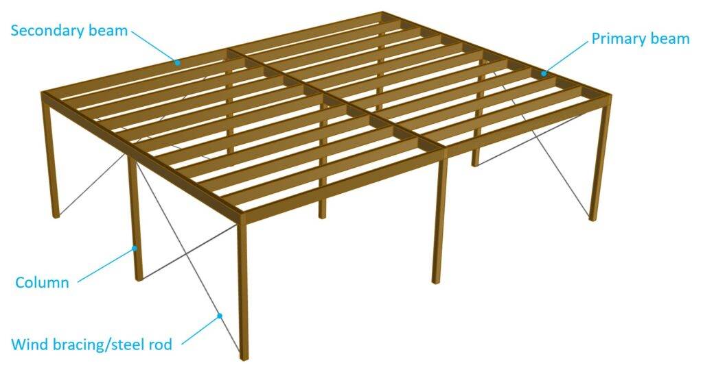
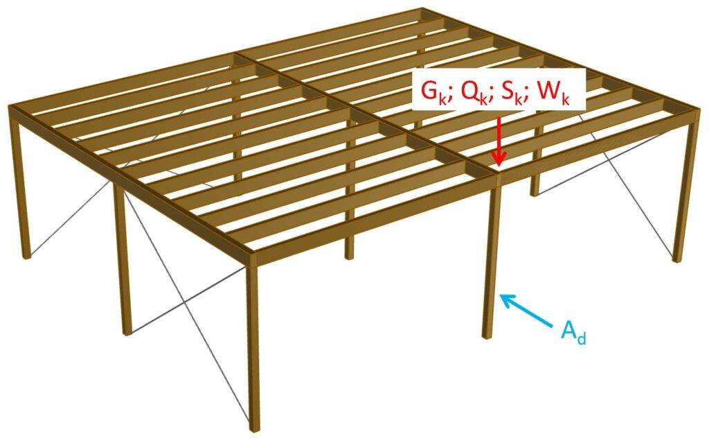
Example Structure For Explanation Of Load Combinations

We’ll show how load combinations work and how to calculate them with the following example structure and example loads.

Example flat roof

First, let’s define some symbols and values for our loads.

gk	1.08 kN/m2	Characteristic value of dead load
qk	1.0 kN/m2	Characteristic value of live load
sk	1.0 kN/m2	Characteristic value of snow load
wk	-1.0 kN/m2	Characteristic value of wind load

ULS Load Combinations

ULS stands for ultimate limit state. Due to ULS load combinations, structural members are designed for bending, shear, buckling, etc. EN 1990 6.4.3.2 calls ULS load combinations “Combinations of actions for persistent or transient design situations”.

The formula of ULS load combinations is (EN 1990 (6.10)):

With,

• γ_G = Partial factor of the dead load
• G_k = Dead load
• γ_Q.1 = Partial factor of the leading variable action/load like live, snow or wind load
• Q_k.1 = Leading variable action
• γ_Q.i = Partial factor of the accompanying actions/loads like live, snow or wind load
• ψ_0.i = Psi factor of the accompanying actions/loads
• Q_k.i = Accompanying variable action

Partial factors

The partial factors are found in EN 1990 Table A1.2(A), A1.2(B), A1.2(C) and A1.3. Note that these factors might be defined differently in your National Annex.

Action	γ factor
Dead load favourable	γG.inf = 0.9
Dead load unfavourable	γG.sup = 1.35
Variable actions (live, snow, wind load)	γQ = 1.5

ψ₀ factors

We find the ψ factors in EN 1990 Table A1.1. Please be aware that every country might define these factors differently in its National Annex.

Action	ψ0
Cat. A: domestic, residential areas	0.7
Cat. B: office areas	0.7
Cat. C: congregation areas	0.7
Cat. D: shopping areas	0.7
Cat. E: storage areas	1.0
Cat. F: traffic area, vehicle weight < 30 kN	0.7
Cat. G: traffic area, 30 kN < vehicle weight < 160 kN	0.7
Cat. H: roofs	0
Snow loads (Finland, Iceland, Norway, Sweden)	0.7
Snow loads (Other CEN member states, for sites located at altitude H < 1000m)	0.7
Snow loads (Other CEN member states, for sites located at altitude H > 1000m)	0.5
Wind loads	0.6

ULS load combinations applied to example structure

According to Eurocode EN 1990 (6.10) in our example the load combinations can be written as:

LC1	$\gamma_{g} \cdot g_{k} $
LC2	$\gamma_{g} \cdot g_{k} + \gamma_{q} \cdot q_{k}$
LC3	$\gamma_{g} \cdot g_{k} + \gamma_{q} \cdot q_{k} + \Psi_{0.s} \cdot \gamma_{q} \cdot s_{k}$
LC4	$\gamma_{g} \cdot g_{k} + \Psi_{0.q} \cdot \gamma_{q} \cdot q_{k} + \gamma_{q} \cdot s_{k}$
LC5	$\gamma_{g} \cdot g_{k} + \gamma_{q} \cdot q_{k} + \Psi_{0.s} \cdot \gamma_{q} \cdots_{k} + \Psi_{0.w} \cdot \gamma_{q} \cdot w_{k} $
LC6	$\gamma_{g} \cdot g_{k} + \Psi_{0.q} \cdot \gamma_{q} \cdot q_{k} + \gamma_{q} \cdot s_{k} + \Psi_{0.w} \cdot \gamma_{q} \cdot w_{k} $
LC7	$\gamma_{g} \cdot g_{k} + \Psi_{0.q} \cdot \gamma_{q} \cdot q_k + \Psi_{0.s} \cdot \gamma_{q} \cdot s_{k} + \gamma_{q} \cdot w_{k} $
LC8	$\gamma_{g} \cdot g_{k} + \gamma_{q} \cdot s_{k} $
LC9	$\gamma_{g} \cdot g_{k} + \gamma_{q} \cdot w_{k} $
LC10	$\gamma_{g} \cdot g_{k} + \gamma_{q} \cdot s_{k} + \Psi_{0.w} \cdot \gamma_{q} \cdot w_{k} $
LC11	$\gamma_{g} \cdot g_{k} + \gamma_{q} \cdot w_{k} + \Psi_{0.s} \cdot \gamma_{q} \cdot s_{k} $
LC12	$\gamma_{g} \cdot g_{k} + \gamma_{q} \cdot q_{k} + \Psi_{0.w} \cdot \gamma_{q} \cdot w_{k}$
LC13	$\gamma_g \cdot g_k + \gamma_q \cdot \Psi_{0.q} \cdot q_k + \gamma_{q} \cdot w_{k}$
LC14	$\gamma_{g.inf} \cdot g_k + \gamma_q \cdot w_k$

Where

$\gamma_{g}$	Partial factor for permanent loads from EN 1990 Table A1.2(B)
$\gamma_{q}$	Partial factor for variable loads from EN 1990 Table A1.2(B)
$\gamma_{g.inf}$	Partial factor for permanent loads (lower value) from EN 1990 Table A1.2(B)
$\Psi_{0.q}$	Factor for combination value of live load from EN 1990 Table A1.1
$\Psi_{0.s}$	Factor for combination value of snow load from EN 1990 Table A1.1
$\Psi_{0.w}$	Factor for combination value of wind load from EN 1990 Table A1.1

For the case of the flat roof, we get the following values for ψ₀– and γ-factor:

$\gamma_{g}$	1.35 (unfavourable)
$\gamma_{q}$	1.5
$\Psi_{0.q}$	0
$\Psi_{0.s}$	0.7 (Sweden)
$\Psi_{0.w}$	0.6

These values we can now put in the load combinations.

LC1	$1.35 \cdot 1.08 \frac{kN}{m^2} $	$1.46 \frac{kN}{m^2}$
LC2	$1.35 \cdot 1.08 \frac{kN}{m^2} + 1.5 \cdot 1.0 \frac{kN}{m^2}$	$2.96 \frac{kN}{m^2} $
LC3	$1.35 \cdot 1.08 \frac{kN}{m^2} + 1.5 \cdot 1.0 \frac{kN}{m^2} + 0.7 \cdot 1.5 \cdot 1.0 \frac{kN}{m^2}$	$4.0 \frac{kN}{m^2}$
LC4	$1.35 \cdot 1.08 \frac{kN}{m^2} + 0 \cdot 1.5 \cdot 1.0 \frac{kN}{m^2} + 1.5 \cdot 1.0 \frac{kN}{m^2}$	$2.96 \frac{kN}{m^2} $
LC5	$1.35 \cdot 1.08 \frac{kN}{m^2} + 1.5 \cdot 1.0 \frac{kN}{m^2} + 0.7 \cdot 1.5 \cdot 1.0 \frac{kN}{m^2} + 0.6 \cdot 1.5 \cdot (-1.0 \frac{kN}{m^2}) $	$3.1 \frac{kN}{m^2}$
LC6	$1.35 \cdot 1.08 \frac{kN}{m^2} + \Psi_{0} \cdot 1.5 \cdot 1.0 \frac{kN}{m^2} + 1.5 \cdot 1.0 \frac{kN}{m^2} + 0.6 \cdot 1.5 \cdot (-1.0 \frac{kN}{m^2}) $	$2.1 \frac{kN}{m^2} $
LC7	$1.35 \cdot 1.08 \frac{kN}{m^2} + 0 \cdot 1.5 \cdot 1.0 \frac{kN}{m^2} + 0.7 \cdot 1.5 \cdot 1.0 \frac{kN}{m^2} + 1.5 \cdot (-1.0 \frac{kN}{m^2}) $	$1.0 \frac{kN}{m^2}$
LC8	$1.35 \cdot 1.08 \frac{kN}{m^2} + 1.5 \cdot 1.0 \frac{kN}{m^2} $	$ 2.96 \frac{kN}{m^2} $
LC9	$1.35 \cdot 1.08 \frac{kN}{m^2} + 1.5 \cdot (-1.0 \frac{kN}{m^2}) $	$ -0.04 \frac{kN}{m^2} $
LC10	$1.35 \cdot 1.08 \frac{kN}{m^2} + 1.5 \cdot 1.0 \frac{kN}{m^2} + 0.6 \cdot 1.5 \cdot (-1.0 \frac{kN}{m^2}) $	$ 2.06 \frac{kN}{m^2}$
LC11	$1.35 \cdot 1.08 \frac{kN}{m^2} + 1.5 \cdot (-1.0 \frac{kN}{m^2}) + 0.7 \cdot 1.5 \cdot 1.0 \frac{kN}{m^2} $	$1.0 \frac{kN}{m^2}$
LC12	$1.35 \cdot 1.08 \frac{kN}{m^2} + 1.5 \cdot 1.0 \frac{kN}{m^2} + 0.6 \cdot 1.5 \cdot (-1.0 \frac{kN}{m^2})$	$2.06 \frac{kN}{m^2}$
LC13	$1.35 \cdot 1.08 \frac{kN}{m^2} + 1.5 \cdot 0 \cdot 1.0 \frac{kN}{m^2} + 1.5 \cdot (-1.0 \frac{kN}{m^2}) $	$-0.04 \frac{kN}{m^2}$
LC14	$1.0 \cdot 1.08 \frac{kN}{m^2} + 1.5 \cdot \frac{kN}{m^2} + 1.5 \cdot (-1.0 \frac{kN}{m^2})$	$-0.42 \frac{kN}{m^2}$

Don’t worry, you do not have to do this manually every time because luckily most FE programs do that for us.

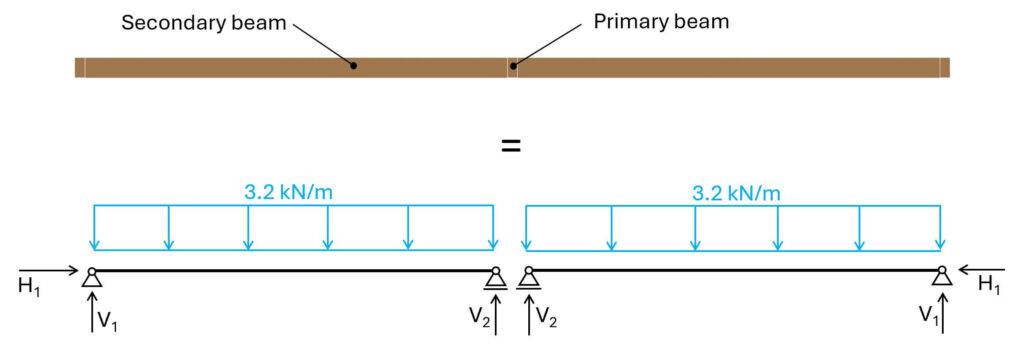
But if we were to dimension a timber beam for bending now manually we would use the biggest value of the load combinations which is 4.0 kN/m² (LC3) and transform it first in a line load (kN/m).

Assuming that the beams have a spacing of 0.8m we get the following line load:

That line load can now be applied to the static system of the secondary beams.

Accidental Load Combinations

According to EN 1990 1.5.3.5 an accidental action is defined as:

Action, usually of short duration but of significant magnitude, that is unlikely to occur on a given structure during the design working life.

Example of accidental design situations are a fire, an explosion, impact loads from vehicles or the consequences of localised failure.

The formula of accidental combinations is (EN 1990 (6.11b)):

With,

• G_k = Dead load
• A_d = Accidental action/load like e.g. impact load from vehicle
• Q_k.1 = Leading variable action
• ψ_1.i or ψ_2.i = Psi factors of the variable actions/loads
• Q_k.i = Accompanying variable actions

Action	ψ1	ψ2
Cat. A: domestic, residential areas	0.5	0.3
Cat. B: office areas	0.5	0.3
Cat. C: congregation areas	0.7	0.6
Cat. D: shopping areas	0.7	0.6
Cat. E: storage areas	0.9	0.8
Cat. F: traffic area, vehicle weight < 30 kN	0.7	0.6
Cat. G: traffic area, 30 kN < vehicle weight < 160 kN	0.5	0.3
Cat. H: roofs	0.0	0.0
Snow loads (Finland, Iceland, Norway, Sweden)	0.5	0.2
Snow loads (Other CEN member states, for sites located at altitude H < 1000m)	0.5	0.2
Snow loads (Other CEN member states, for sites located at altitude H > 1000m)	0.2	0.0
Wind loads	0.2	0.0

Accidental load combinations applied to example structure

Let’s say the accidental action is an impact load from a car that crashes into one of the columns of the carport.

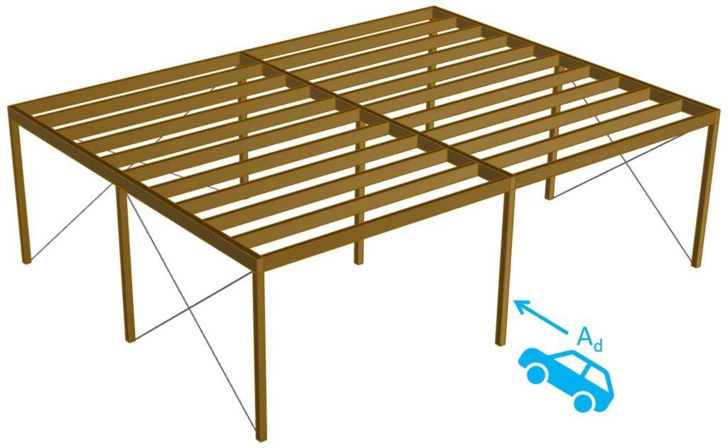
According to our article about impact loads from vehicles the accidental action A_d is defined as:

Now, let’s assume that the characteristic vertical loads on the column are:

Gk	9.0 kN	Characteristic value of dead load
Qk	8.0 kN	Characteristic value of live load
Sk	8.0 kN	Characteristic value of snow load
Wk	-8.0 kN	Characteristic value of wind load

According to Eurocode EN 1990 (6.11b) in our example the load combinations can be written as:

LC1	$G_{k} + A_d + \Psi_{1.q} \cdot Q_{k}$
LC2	$G_{k} + A_d + \Psi_{1.q} \cdot Q_{k} + \Psi_{2.s} \cdot S_{k}$
LC3	$G_{k} + A_d + \Psi_{1.q} \cdot Q_{k} + \Psi_{2.w} \cdot W_{k}$
LC4	$G_{k} + A_d + \Psi_{1.q} \cdot Q_{k} + \Psi_{2.w} \cdot W_{k} + \Psi_{2.s} \cdot S_{k}$
LC5	$G_{k} + A_d + \Psi_{1.s} \cdot S_{k} + \Psi_{2.q} \cdot Q_{k}$
LC6	$G_{k} + A_d + \Psi_{1.s} \cdot S_{k} + \Psi_{2.w} \cdot W_{k}$
LC7	$G_{k} + A_d + \Psi_{1.s} \cdot S_{k} + \Psi_{2.w} \cdot W_{k} + \Psi_{2.q} \cdot Q_{k}$
LC8	$G_{k} + A_d + \Psi_{1.w} \cdot W_{k} + \Psi_{2.q} \cdot Q_{k}$
LC9	$G_{k} + A_d + \Psi_{1.w} \cdot W_{k} + \Psi_{2.s} \cdot S_{k}$
LC10	$G_{k} + A_d + \Psi_{1.w} \cdot W_{k} + \Psi_{2.s} \cdot S_{k} + \Psi_{2.q} \cdot Q_{k}$

Now, you can go ahead and design the timber column for the horizontal and vertical design load.

Seismic Load Combinations

Seismic actions and load combinations are the result of earthquakes. In many parts of the world this is the leading horizontal design load acting on a building and in other parts the seismic load is much smaller than the horizontal wind load.

The formula of accidental combinations is (EN 1990 (6.12b)):

With,

• G_k = Dead load
• A_Ed = Design value of seismic action
• Q_k.i = Variable actions
• ψ_2.i = Psi factors of the variable actions/loads

Seismic load combinations applied to example structure

According to Eurocode EN 1990 (6.12b) in our example the load combinations can be written as:

LC1	$G_{k} + A_{Ed} + \Psi_{2.q} \cdot Q_{k}$
LC2	$G_{k} + A_{Ed} + \Psi_{2.q} \cdot Q_{k} + \Psi_{2.s} \cdot S_{k}$
LC3	$G_{k} + A_{Ed} + \Psi_{2.q} \cdot Q_{k} + \Psi_{2.w} \cdot W_{k}$
LC4	$G_{k} + A_{Ed} + \Psi_{2.q} \cdot Q_{k} + \Psi_{2.w} \cdot W_{k} + \Psi_{2.s} \cdot S_{k}$
LC5	$G_{k} + A_{Ed} + \Psi_{2.s} \cdot S_{k} + \Psi_{2.q} \cdot Q_{k}$
LC6	$G_{k} + A_{Ed} + \Psi_{2.s} \cdot S_{k} + \Psi_{2.w} \cdot W_{k}$
LC7	$G_{k} + A_{Ed} + \Psi_{2.s} \cdot S_{k} + \Psi_{2.w} \cdot W_{k} + \Psi_{2.q} \cdot Q_{k}$
LC8	$G_{k} + A_{Ed} + \Psi_{2.w} \cdot W_{k} + \Psi_{2.q} \cdot Q_{k}$
LC9	$G_{k} + A_{Ed} + \Psi_{2.w} \cdot W_{k} + \Psi_{2.s} \cdot S_{k}$
LC10	$G_{k} + A_{Ed} + \Psi_{2.w} \cdot W_{k} + \Psi_{2.s} \cdot S_{k} + \Psi_{2.q} \cdot Q_{k}$

SLS Characteristic Load Combinations

SLS stands for serviceability limit state. Due to SLS characteristic load combinations structural members are designed for example for deflection.

The formula of SLS characteristic combinations is (EN 1990 (6.14b)):

With,

• G_k = Dead load
• Q_k.1 = Leading variable action
• ψ_0.i = Psi factor of the accompanying actions/loads
• Q_k.i = Accompanying variable action

SLS characteristic load combinations applied to example structure

According to EN 1990 (6.14b) the characteristic load combinations can be written as:

LC1	$g_{k} $
LC2	$g_{k} + q_{k}$
LC3	$g_{k} + q_{k} + \Psi_{0.s} \cdot s_{k}$
LC4	$g_{k} + q_{k} + \Psi_{0.w} \cdot w_{k}$
LC5	$g_{k} + q_{k} + \Psi_{0.s} \cdot s_{k} + \Psi_{0.w} \cdot w_{k} $
LC6	$g_{k} + \Psi_{0.q} \cdot q_{k} + s_{k} + \Psi_{0.w} \cdot w_{k} $
LC7	$g_{k} + \Psi_{0.q} \cdot q_{k} + \Psi_{0.s} \cdot s_{k} + w_{k} $
LC8	$g_{k} + s_{k} $
LC9	$g_{k} + w_{k} $
LC10	$g_{k} + s_{k} + \Psi_{0.w} \cdot w_{k} $
LC11	$g_{k} + w_{k} + \Psi_{0.s} \cdot s_{k} $
LC12	$g_{k} + \Psi_{0.q} \cdot q_{k} + s_{k}$
LC13	$g_{k} + \Psi_{0.q} \cdot q_{k} + w_{k}$

And if we put in the values, we get ..

LC1	$1.08 \frac{kN}{m^2} $	$1.08 \frac{kN}{m^2}$
LC2	$1.08 \frac{kN}{m^2} + 1.0 \frac{kN}{m^2}$	$2.08 \frac{kN}{m^2}$
LC3	$1.08 \frac{kN}{m^2} + 1.0 \frac{kN}{m^2} + 0.7 \cdot 1.0 \frac{kN}{m^2}$	$2.78 \frac{kN}{m^2}$
LC4	$1.08 \frac{kN}{m^2} + 1.0 \frac{kN}{m^2} + 0.6 \cdot (-1.0 \frac{kN}{m^2})$	$1.48 \frac{kN}{m^2}$
LC5	$1.08 \frac{kN}{m^2} + 1.0 \frac{kN}{m^2} + 0.7 \cdot 1.0 \frac{kN}{m^2} + 0.6 \cdot (-1.0 \frac{kN}{m^2}) $	$2.18 \frac{kN}{m^2}$
LC6	$1.08 \frac{kN}{m^2} + 0 \cdot 1.0 \frac{kN}{m^2} + 1.0 \frac{kN}{m^2} + 0.6 \cdot (-1.0 \frac{kN}{m^2}) $	$1.48 \frac{kN}{m^2}$
LC7	$1.08 \frac{kN}{m^2} + 0 \cdot 1.0 \frac{kN}{m^2} + 0.7 \cdot 1.0 \frac{kN}{m^2} + (-1.0 \frac{kN}{m^2}) $	$0.78 \frac{kN}{m^2}$
LC8	$1.08 \frac{kN}{m^2} + 1.0 \frac{kN}{m^2}$	$2.08 \frac{kN}{m^2}$
LC9	$1.08 \frac{kN}{m^2} + (-1.0 \frac{kN}{m^2}) $	$0.08 \frac{kN}{m^2}$
LC10	$1.08 \frac{kN}{m^2} + 1.0 \frac{kN}{m^2} + 0.6 \cdot (-1.0 \frac{kN}{m^2}) $	$1.48 \frac{kN}{m^2}$
LC11	$1.08 \frac{kN}{m^2} + (-1.0 \frac{kN}{m^2}) + 0.7 \cdot 1.0 \frac{kN}{m^2} $	$0.78 \frac{kN}{m^2}$
LC12	$1.08 \frac{kN}{m^2} + 0 \cdot 1.0 \frac{kN}{m^2} + 1.0 \frac{kN}{m^2}$	$2.08 \frac{kN}{m^2}$
LC13	$1.08 \frac{kN}{m^2} + 0 \cdot 1.0 \frac{kN}{m^2} + (-1.0 \frac{kN}{m^2})$	$0.08 \frac{kN}{m^2}$

Now let’s move on to the quasi-permanent SLS load combination.

SLS Quasi-Permanent Combination

The SLS quasi-permanent load combinations are used to calculate for example the quasi-permanent moment which is used to verify cracking of reinforced concrete beams or rc slabs.

The formula of SLS quasi-permanent combinations is (EN 1990 (6.16b)):

With,

• G_k = Dead load
• Q_k.i = Variable actions
• ψ_2.i = Psi factor of variable actions/loads

SLS quasi-permanent load combinations applied to example structure

According to EN 1990 (6.16b) in our example the quasi-permanent load combinations can be written as.

LC1	$g_{k} $
LC2	$g_{k} + \Psi_{2.q} \cdot q_{k}$
LC3	$g_{k} + \Psi_{2.q} \cdot q_{k} + \Psi_{2.s} \cdot s_{k}$
LC4	$g_{k} + \Psi_{2.q} \cdot q_{k} + \Psi_{2.w} \cdot w_{k}$
LC5	$g_{k} + \Psi_{2.q} \cdot q_{k} + \Psi_{2.s} \cdot s_{k} + \Psi_{2.w} \cdot w_{k} $
LC6	$g_{k} + \Psi_{2.s} \cdot s_{k} $
LC7	$g_{k} + \Psi_{2.w} \cdot w_{k} $
LC8	$g_{k} + \Psi_{2.s} \cdot s_{k} + \Psi_{2.w} \cdot w_{k} $

Where

$\Psi_{2.q}$	0
$\Psi_{2.s}$	0.2 (Sweden)
$\Psi_{2.w}$	0

And if we put in the values, we will get ..

LC1	$1.08 \frac{kN}{m^2} $	$1.08 \frac{kN}{m^2} $
LC2	$1.08 \frac{kN}{m^2} + 0 \cdot 1.0 \frac{kN}{m^2}$	$1.08 \frac{kN}{m^2} $
LC3	$1.08 \frac{kN}{m^2} + 0 \cdot 1.0 \frac{kN}{m^2} + 0.2 \cdot 1.0 \frac{kN}{m^2}$	$1.28 \frac{kN}{m^2} $
LC4	$1.08 \frac{kN}{m^2} + 0 \cdot 1.0 \frac{kN}{m^2} + 0 \cdot (-1.0 \frac{kN}{m^2})$	$1.08 \frac{kN}{m^2} $
LC5	$1.08 \frac{kN}{m^2} + 0 \cdot 1.0 \frac{kN}{m^2} + 0.2 \cdot 1.0 \frac{kN}{m^2} + 0 \cdot (-1.0 \frac{kN}{m^2}) $	$1.28 \frac{kN}{m^2} $
LC6	$1.08 \frac{kN}{m^2} + 0.2 \cdot 1.0 \frac{kN}{m^2} $	$1.28 \frac{kN}{m^2} $
LC7	$1.08 \frac{kN}{m^2} + 0 \cdot (-1.0 \frac{kN}{m^2}) $	$1.08 \frac{kN}{m^2} $
LC8	$1.08 \frac{kN}{m^2} + 0.2 \cdot 1.0 \frac{kN}{m^2} + 0 \cdot (-1.0 \frac{kN}{m^2}) $	$1.28 \frac{kN}{m^2} $

SLS Frequent Combination

The formula of SLS frequent combinations is (EN 1990 (6.15b)):

With,

• G_k = Dead load
• Q_k.1 = Leading variable action
• ψ_1.i = Frequent psi factor of the leading variable action/load
• Q_k.i = Accompanying variable action
• ψ_2.i = Quasi-permanent psi factor of the accompanying variable action/load

SLS frequent load combinations applied to example structure

According to EN 1990 (6.15b) in our example the quasi-permanent load combinations can be written as.

LC1	$g_{k} + \Psi_{1.q} \cdot q_{k}$
LC2	$g_{k} + \Psi_{1.q} \cdot q_{k} + \Psi_{2.s} \cdot s_{k}$
LC3	$g_{k} + \Psi_{1.q} \cdot q_{k} + \Psi_{2.w} \cdot w_{k}$
LC4	$g_{k} + \Psi_{1.q} \cdot q_{k} + \Psi_{2.w} \cdot w_{k} + \Psi_{2.s} \cdot s_{k}$
LC5	$g_{k} + \Psi_{1.s} \cdot s_{k} + \Psi_{2.q} \cdot q_{k}$
LC6	$g_{k} + \Psi_{1.s} \cdot s_{k} + \Psi_{2.w} \cdot w_{k}$
LC7	$g_{k} + \Psi_{1.s} \cdot s_{k} + \Psi_{2.w} \cdot w_{k} + \Psi_{2.q} \cdot q_{k}$
LC8	$g_{k} + \Psi_{1.w} \cdot w_{k} + \Psi_{2.q} \cdot q_{k}$
LC9	$g_{k} + \Psi_{1.w} \cdot w_{k} + \Psi_{2.s} \cdot s_{k}$
LC10	$g_{k} + \Psi_{1.w} \cdot w_{k} + \Psi_{2.s} \cdot s_{k} + \Psi_{2.q} \cdot q_{k}$

Conclusion

Load combinations are a very important part of structural design. Back when I was still studying at uni, I realized that many of my fellow students had problems understanding how load combinations work.

That’s because there isn’t really a course dedicated to load combinations. At most unis you have to learn it yourself.

But it’s really dangerous if you don’t calculate the design loads correctly with load combinations because ultimately you design your element with wrong loads.

I hope this guide helps to understand load combinations better.

To learn more about structural engineering you can also check out:

• Design of reinforced concrete beams
• Wind loads on walls explained
• What’s the difference between statically determinate and indeterminate structures?

Load Combinations FAQ